
K-Means
- Rows
- Every row gets a cluster.
- Center
- A mean centroid.
- Distance
- Euclidean.
- Complexity
- O(n·k·d·i)
Loading…
A centroid is the mean of the rows in its cluster, so the center can sit between customers. Hierarchical clustering merges those rows by a linkage until the cut leaves k groups, and that cut does not fit a centroid.
Choose whether the groups come from a mean or from a cut.
This is a choice, not a measured winner.
K-Means Clustering has the higher silhouette on Iris Flowers and Customer Segments; Silhouette is within 0.01 on Wine (UCI wine recognition).
Should the groups come from a merge and a cut?
A linkage builds the tree, and the cut leaves k groups.
Wholesale Customers has 440 rows and six spend columns: Fresh, Milk, Grocery, Frozen, Detergents_Paper, and Delicassen. Channel and Region stay out of the fit.
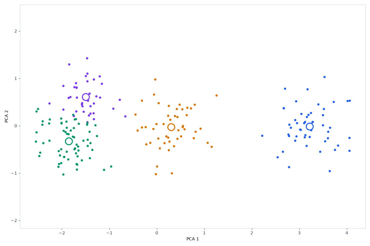
K-Means has 3 clusters. Silhouette 0.548287. Calinski–Harabasz 140.135183. Davies–Bouldin 0.927935. Inertia 1608.431149. Adjusted Rand —.
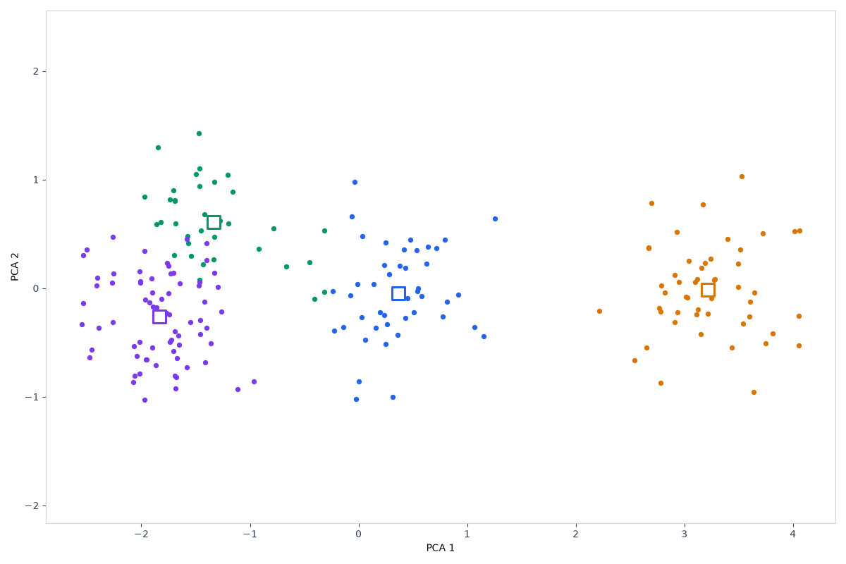
Ward has 3 clusters. Silhouette 0.264609. Calinski–Harabasz 111.151039. Davies–Bouldin 1.284521. Adjusted Rand —.
On the PCA plot, most customers sit in a dense group and a few sit far out on the tail.
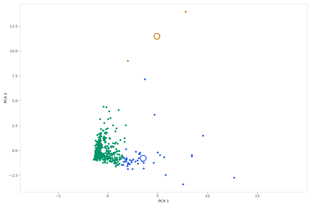
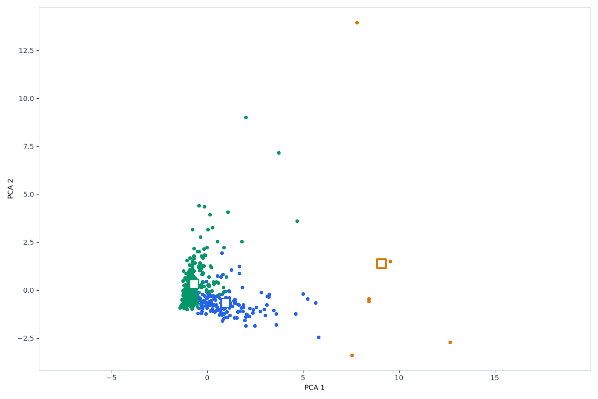
The six spend columns are right-skewed, so a mean can be pulled by the tail, while the Ward cut leaves 3 groups with silhouette 0.264609 against K-Means silhouette 0.548287 on 3 clusters.
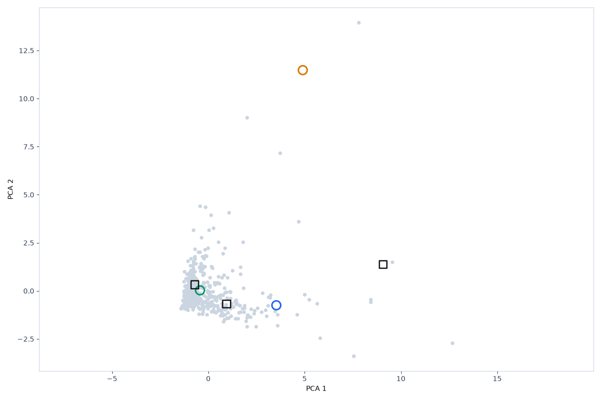
The link loads the six-column sample. K-Means is set to k=3. Hierarchical clustering is set to k=3 and linkage ward. Run is still required.
from sklearn.cluster import KMeans
from sklearn.preprocessing import StandardScaler
Xs = StandardScaler().fit_transform(X)
labels = KMeans(n_clusters=3, n_init=10, random_state=42).fit_predict(Xs)
from sklearn.cluster import AgglomerativeClustering
from sklearn.preprocessing import StandardScaler
Xs = StandardScaler().fit_transform(X)
labels = AgglomerativeClustering(n_clusters=3, linkage='ward').fit_predict(Xs)
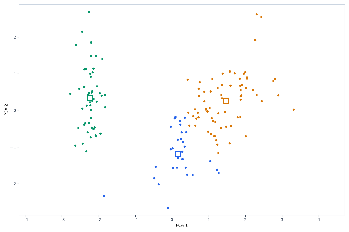
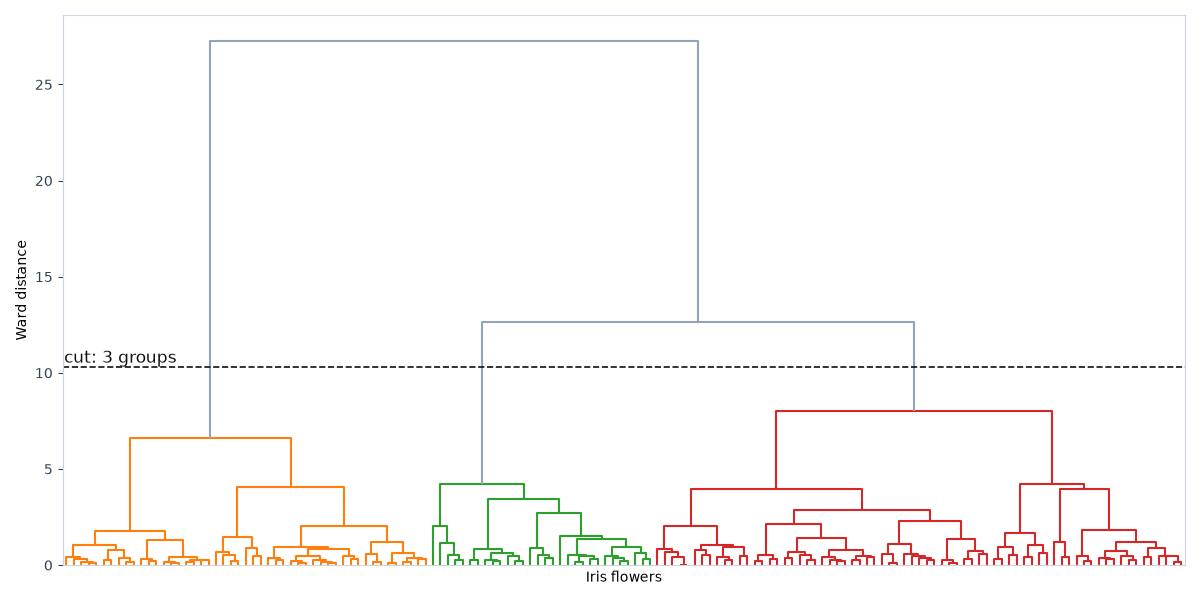
Ward agglomerative clustering on Iris Flowers (150 rows and 4 features) stops at 3 clusters. Its silhouette is 0.447 and its Davies-Bouldin index is 0.803. K-Means on the same table uses 3 centroids, silhouette 0.460, Davies-Bouldin 0.834. The flat centroid fit separates these rows more cleanly than the Ward merge.
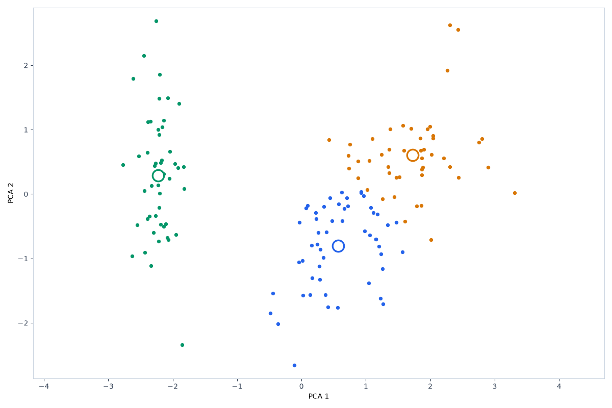
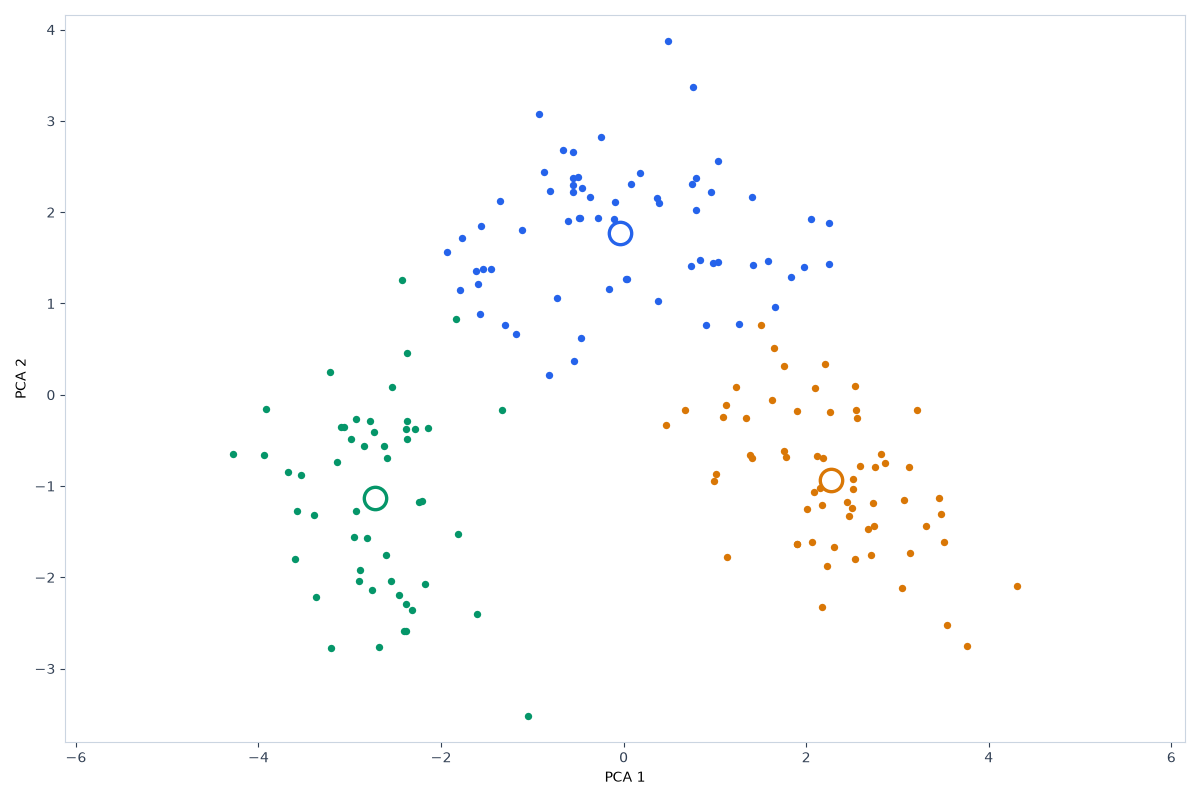
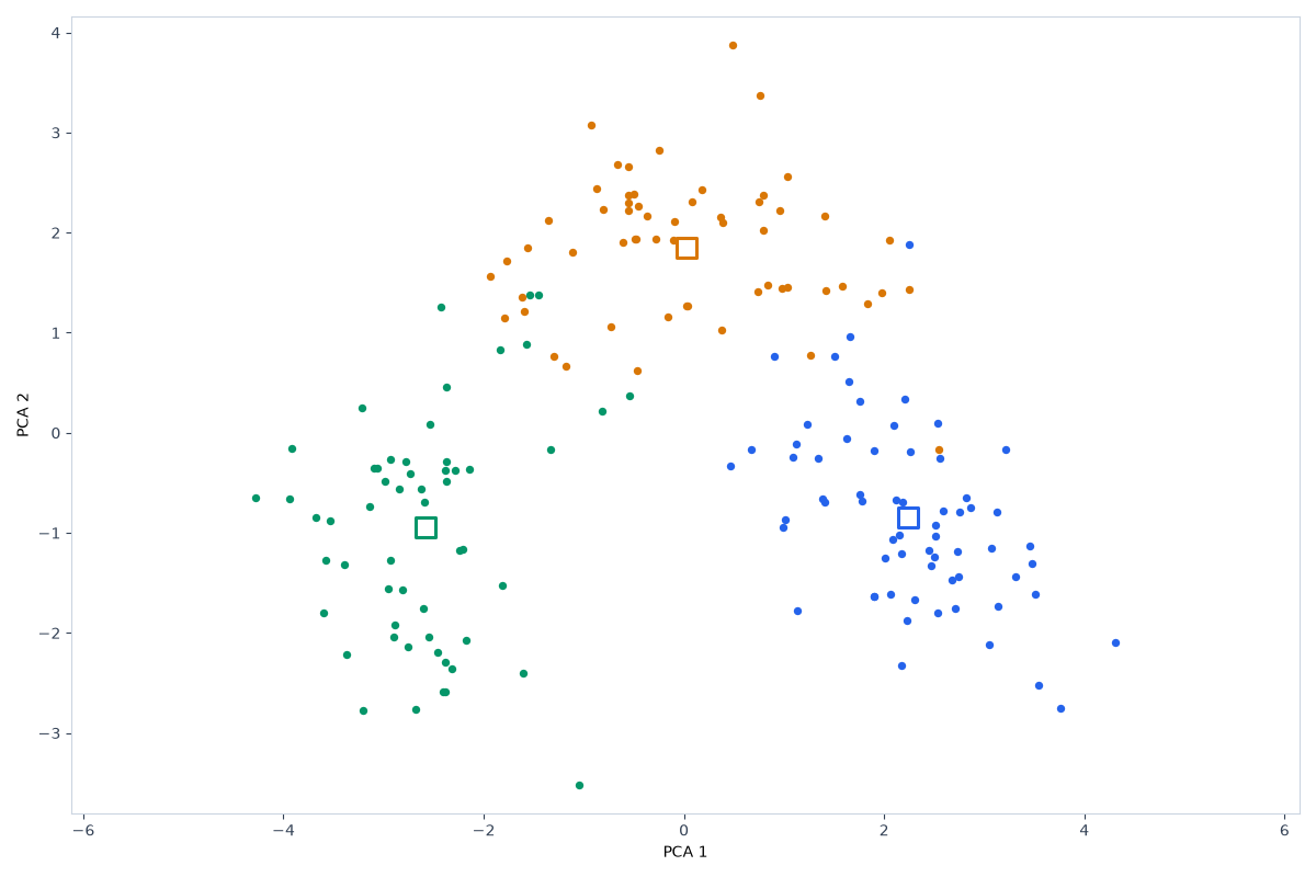
Ward agglomerative clustering on Wine (UCI wine recognition) (178 rows and 13 features) stops at 3 clusters. Its silhouette is 0.277 and its Davies-Bouldin index is 1.419. K-Means on the same table uses 3 centroids, silhouette 0.285, Davies-Bouldin 1.389. The Ward merge and the centroid fit are too close to call on silhouette.
Silhouette is within 0.01 on Wine because this hierarchical fit uses Ward linkage, which merges clusters to reduce within-cluster variance, the same quantity K-Means iterates on.
Ward agglomerative clustering on Customer Segments (200 rows and 5 features) stops at 4 clusters. Its silhouette is 0.357 and its Davies-Bouldin index is 1.150. K-Means on the same table uses 4 centroids, silhouette 0.368, Davies-Bouldin 1.126. The flat centroid fit separates these rows more cleanly than the Ward merge.
| Dataset | Algorithm | Clusters | Noise | Silhouette | Adjusted Rand |
|---|---|---|---|---|---|
| Wholesale Customers | K-Means | 3 | 0 | 0.548 | — |
| Wholesale Customers | Hierarchical clustering | 3 | 0 | 0.265 | — |
| Iris Flowers | K-Means Clustering | 3 | 0 | 0.460 | 0.620 |
| Iris Flowers | Agglomerative Hierarchical Clustering | 3 | 0 | 0.447 | 0.615 |
| Wine (UCI wine recognition) | K-Means Clustering | 3 | 0 | 0.285 | 0.897 |
| Wine (UCI wine recognition) | Agglomerative Hierarchical Clustering | 3 | 0 | 0.277 | 0.790 |
| Customer Segments | K-Means Clustering | 4 | 0 | 0.368 | 0.763 |
| Customer Segments | Agglomerative Hierarchical Clustering | 4 | 0 | 0.357 | 0.708 |
A centroid is the mean of the rows in its cluster, so the center can sit between customers. Hierarchical clustering merges those rows by a linkage until the cut leaves k groups, and that cut does not fit a centroid.
This is a choice, not a measured winner.
The six spend columns are right-skewed, so a mean can be pulled by the tail, while the Ward cut leaves 3 groups with silhouette 0.264609 against K-Means silhouette 0.548287 on 3 clusters.
Method: StandardScaler, drop constant columns. Code version 3e4afc4b4352 (scripts/seo/build_explore_artifacts.py). scikit-learn 1.4.2. Seed 42. Both algorithms were fit on the same scaled table. Where a label column exists, it was held out of the fit and scored with adjusted Rand. Iris Flowers: UCI Machine Learning Repository, Iris (Fisher, 1936). License: CC BY 4.0. Wine (UCI wine recognition): UCI Machine Learning Repository, wine recognition. License: CC BY 4.0. Customer Segments: Synthetic customer records bundled with this site. License: Generated for demos; no external license.
Results computed, published, and last updated on 2026-11-02.
The comparison sentences are filled from these published runs by a fixed template, so the scores can be checked against the same datasets in the tool.
Maintainer: nikolaou1982.
Contact: nick1982100@gmail.com.