
DBSCAN
- Neighborhood
- One eps and min_samples.
Loading…
DBSCAN uses one eps for the whole table, so every neighborhood on that table is the same size. OPTICS orders the rows by reachability, so a cluster can be read from a valley in that order on the same rows.
Choose whether a cluster is read from one eps.
This is a choice, not a measured winner.
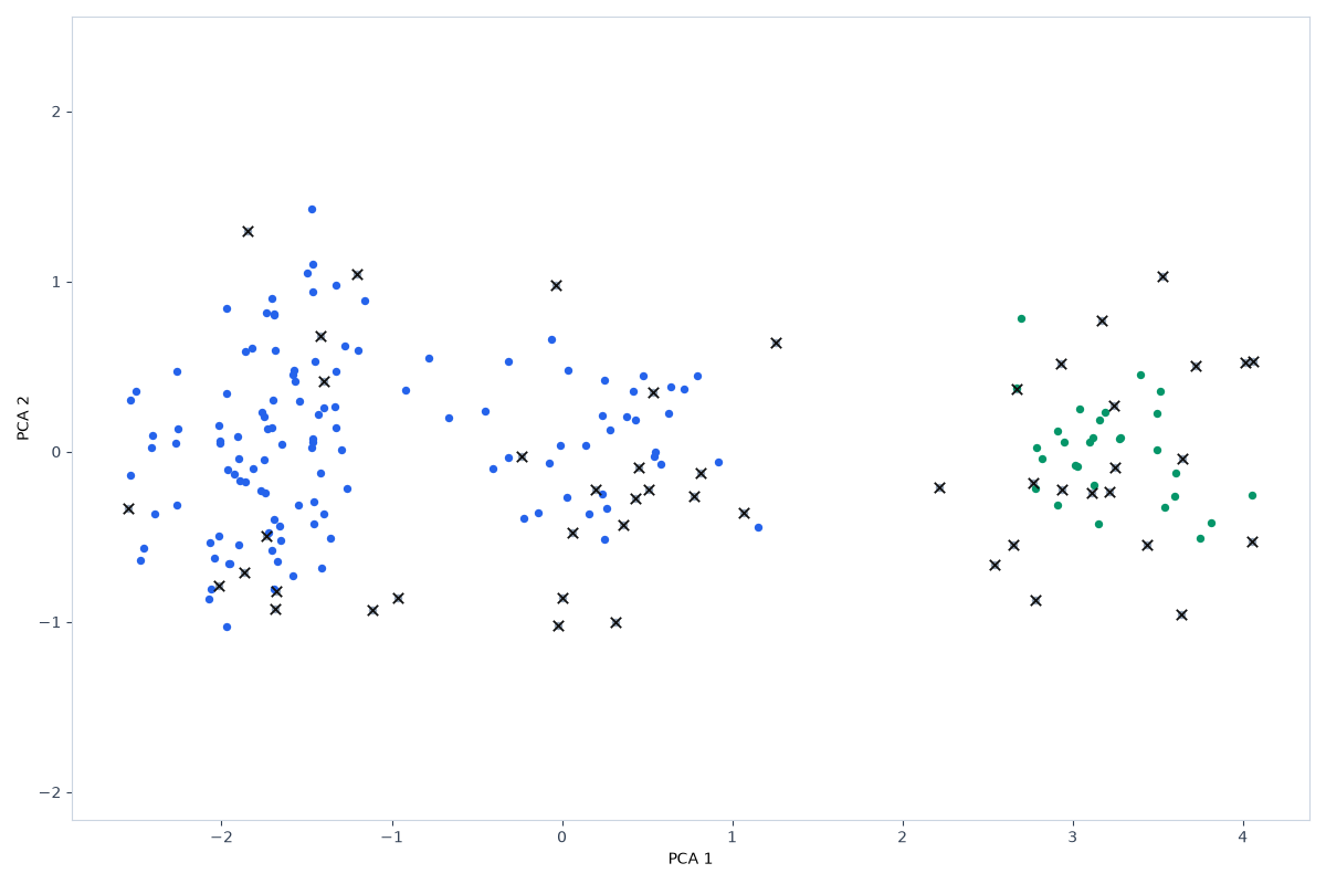
OPTICS Clustering has the higher silhouette on Iris Flowers and Customer Segments; DBSCAN Clustering has no silhouette on Wine (UCI wine recognition), because that fit did not keep two groups; Noise rows show up on Iris Flowers, Wine (UCI wine recognition), and Customer Segments.
Should a cluster be read from a valley in the reachability order?
An ordering of the rows, instead of one eps for the whole table.
Wholesale Customers has 440 rows and six spend columns: Fresh, Milk, Grocery, Frozen, Detergents_Paper, and Delicassen. Channel and Region stay out of the fit.
DBSCAN, 440 rows, 1 cluster, 32 noise rows.
OPTICS, 440 rows, 10 clusters, 350 noise rows. Silhouette 0.417874.
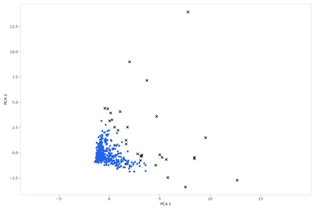
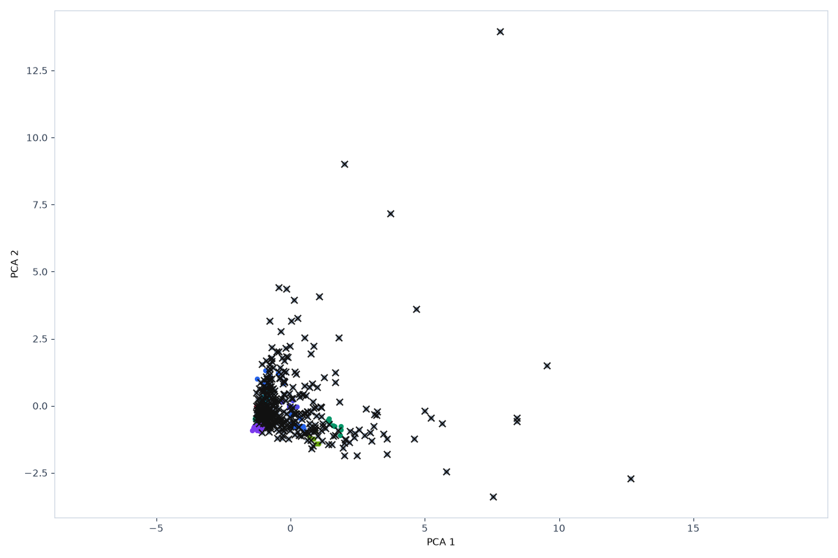
The six spend columns are right-skewed, DBSCAN keeps 1 cluster and marks 32 rows as noise, and OPTICS keeps 10 clusters and marks 350 rows as noise.
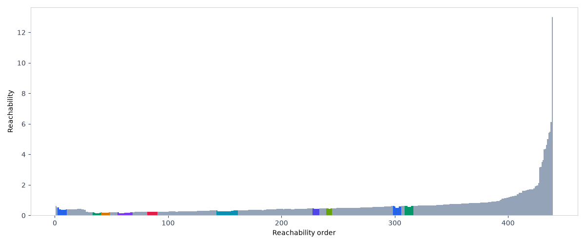
The link loads the six-column sample. DBSCAN is set to eps 1.335645 and min_samples 5. OPTICS is set to min_samples 5 and the xi method. Run is still required.
from sklearn.cluster import DBSCAN
from sklearn.preprocessing import StandardScaler
Xs = StandardScaler().fit_transform(X)
labels = DBSCAN(eps=1.335645, min_samples=5).fit_predict(Xs)
from sklearn.cluster import OPTICS
from sklearn.preprocessing import StandardScaler
Xs = StandardScaler().fit_transform(X)
labels = OPTICS(min_samples=5).fit_predict(Xs)
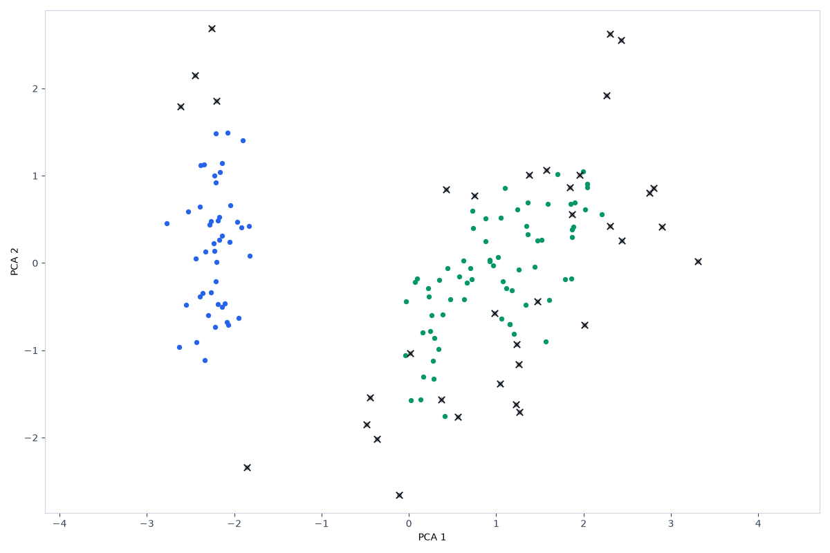
OPTICS on Iris Flowers (150 rows and 4 features) reads 2 clusters out of the reachability order and flags 36 noise rows, silhouette 0.657, Calinski-Harabasz 340.712. DBSCAN, using one epsilon, reads 2 dense regions and flags 4 noise rows, silhouette 0.598, Calinski-Harabasz 277.651. The reachability order separates these rows more cleanly than one epsilon.
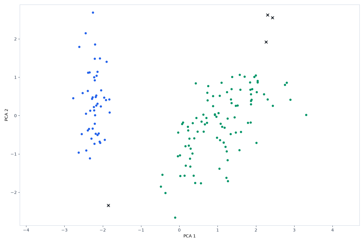
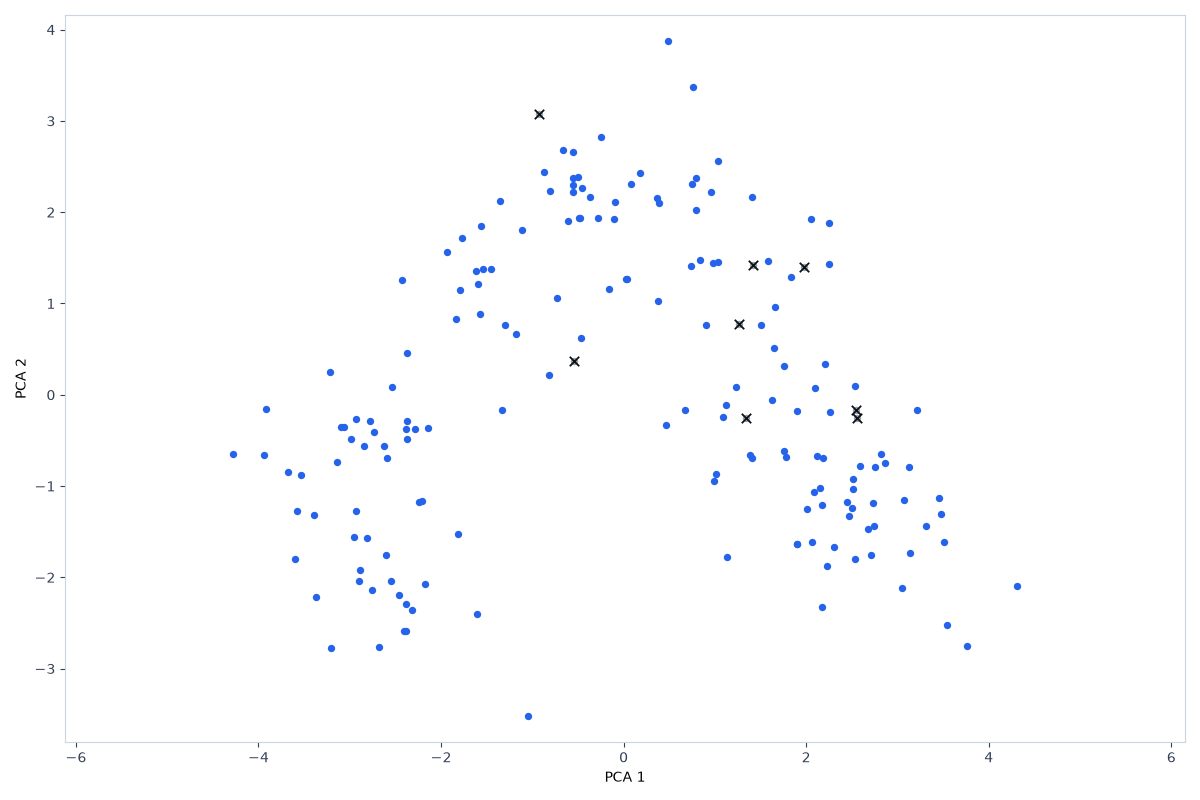
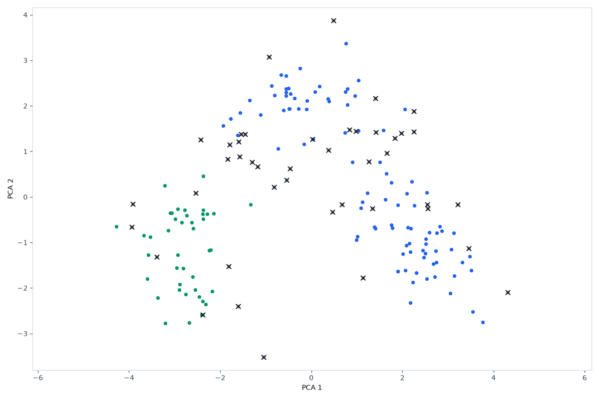
OPTICS on Wine (UCI wine recognition) (178 rows and 13 features) reads 2 clusters out of the reachability order and flags 43 noise rows, silhouette 0.332, Calinski-Harabasz 69.850. DBSCAN, using one epsilon, reads 1 dense regions and flags 8 noise rows, silhouette not defined, Calinski-Harabasz not defined. One epsilon and the reachability order are too close to rank by silhouette.
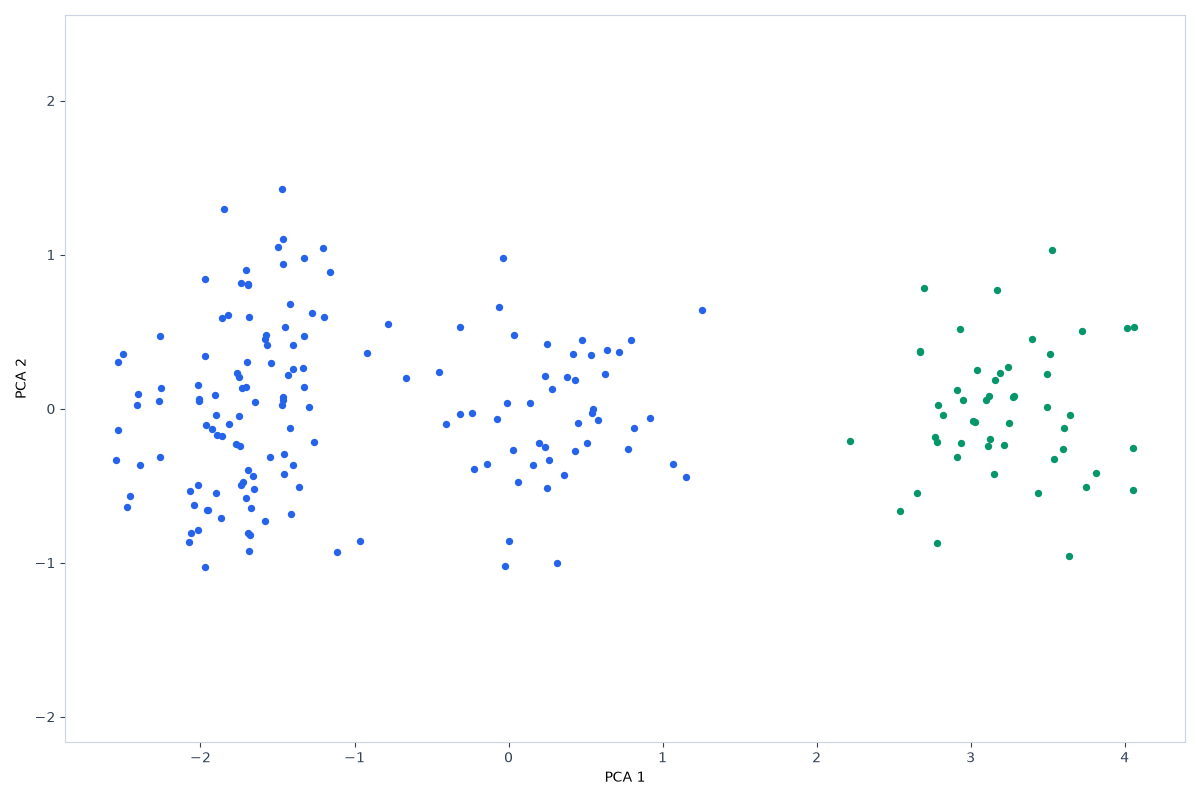
OPTICS on Customer Segments (200 rows and 5 features) reads 2 clusters out of the reachability order and flags 49 noise rows, silhouette 0.650, Calinski-Harabasz 347.613. DBSCAN, using one epsilon, reads 2 dense regions and flags 0 noise rows, silhouette 0.608, Calinski-Harabasz 441.900. The reachability order separates these rows more cleanly than one epsilon.
| Dataset | Algorithm | Clusters | Noise | Silhouette | Adjusted Rand |
|---|---|---|---|---|---|
| Wholesale Customers | DBSCAN | 1 | 32 | — | — |
| Wholesale Customers | OPTICS | 10 | 350 | 0.418 | — |
| Iris Flowers | DBSCAN Clustering | 2 | 4 | 0.598 | 0.552 |
| Iris Flowers | OPTICS Clustering | 2 | 36 | 0.657 | 0.444 |
| Wine (UCI wine recognition) | DBSCAN Clustering | 1 | 8 | not defined | not defined |
| Wine (UCI wine recognition) | OPTICS Clustering | 2 | 43 | 0.332 | 0.392 |
| Customer Segments | DBSCAN Clustering | 2 | 0 | 0.608 | 0.330 |
| Customer Segments | OPTICS Clustering | 2 | 49 | 0.650 | 0.216 |
DBSCAN uses one eps for the whole table, so every neighborhood on that table is the same size. OPTICS orders the rows by reachability, so a cluster can be read from a valley in that order on the same rows.
This is a choice, not a measured winner.
The six spend columns are right-skewed, DBSCAN keeps 1 cluster and marks 32 rows as noise, and OPTICS keeps 10 clusters and marks 350 rows as noise.
Method: StandardScaler, drop constant columns. Code version 3e4afc4b4352 (scripts/seo/build_explore_artifacts.py). scikit-learn 1.4.2. Seed 42. Both algorithms were fit on the same scaled table. Where a label column exists, it was held out of the fit and scored with adjusted Rand. Iris Flowers: UCI Machine Learning Repository, Iris (Fisher, 1936). License: CC BY 4.0. Wine (UCI wine recognition): UCI Machine Learning Repository, wine recognition. License: CC BY 4.0. Customer Segments: Synthetic customer records bundled with this site. License: Generated for demos; no external license.
Results computed, published, and last updated on 2026-11-02.
The comparison sentences are filled from these published runs by a fixed template, so the scores can be checked against the same datasets in the tool.
Maintainer: nikolaou1982.
Contact: nick1982100@gmail.com.